
Application version: 1.0.0
Open source licence: GNU General Public License version 3
Developers: Ebrahim Jahanbakhsh & Michel C. Milinkovitch
Laboratory of Artificial and Natural Evolution (LANE), University of Geneva, Switzerland.
Project website: https://www.lanevol.org/projects/newtonbiomorphx
GitHub: github.com/lanevol/newtonbiomorphx
Original article: NewtonBioMorphX: A computational framework for simulating tissue-scale mechanics of morphogenesis Ebrahim Jahanbakhsh & Michel C. Milinkovitch Computer Physics Communications (2026) (1)
Application logo and icon: Fabrice Berger & Gregory Loichot


The self-organized morphogenesis of multicellular organisms emerges not only from biochemical but also from mechanical processes, operating across spatial scales and producing symmetry breaking through mechanical instabilities. Yet, user-friendly computational tools for simulating tissue-scale mechanics are virtually nonexistent. Over the years, we developed a finite element formulation and applied it to several research projects: the development of a polygonal network of creases in mammalian noses (2); the drug-induced transition from chemical pre-patterning to mechanical skin folding in chicken reticulate scales (3); as well as the self-organized mechanical patterning of scales on the head and jaws of crocodiles (4) and on the top of the head of tortoises (5). These morphogenetic processes are driven by growth and active contractility, and are influenced by the elastic and plastic properties of the tissues, as well as by their anisotropic reinforcement by fibres, multilayer interactions, and curvature.
Here, we present NewtonBioMorphX, a GPU-accelerated, open-source application that brings together all these functionalities within a user-friendly graphical interface. Directly from the interface, you can generate geometries, define material properties, prescribe growth, add anisotropic reinforcement and active forces, visualize results in real time, and export simulations for further analysis.
In short, NewtonBioMorphX makes sophisticated mechanical modeling of morphogenesis accessible without editing or recompiling any code, for biologists and physicists alike. It is also a powerful teaching tool: you can showcase the principles of mechanical patterning, and your students can explore them hands-on themselves.
We encourage you to view the movie (by clicking on the image below), which illustrates the main functionalities of NewtonBioMorphX.

The application has been tested successfully on NVIDIA GPUs with the following CUDA ‘compute capabilities’:
Running the application on pre‑7.0 CUDA architectures may cause significant performance degradation.
Note that the full CUDA Toolkit is not required to run the application: the NVIDIA driver is sufficient.
Ready-to-use versions of NewtonBioMorphX are available on the Releases page of the GitHub repository. Download the file corresponding to your operating system:
| Operating system | File | Description |
|---|---|---|
| Windows | NewtonBioMorphX-<version>-win64.exe |
Installer (recommended) |
| Windows | NewtonBioMorphX-<version>-win64.zip |
Portable version, no installation required |
| Linux | NewtonBioMorphX-x86_64.AppImage |
Single-file executable, no installation required |
Here, <version> stands for the release number (e.g., 1.0.0). We recommend always downloading the latest release.
Installer: double-click NewtonBioMorphX-<version>-win64.exe and follow the instructions. Once installed, NewtonBioMorphX can be launched from the Start menu.
Portable version: unzip NewtonBioMorphX-<version>-win64.zip into any folder (e.g., your Documents folder), then double-click bin\NewtonBioMorphX.exe. Uninstalling simply consists of deleting that folder.
The AppImage is a single file containing the application and its dependencies. Make it executable and launch it from a terminal:
chmod +x NewtonBioMorphX-<version>-x86_64.AppImage
./NewtonBioMorphX-<version>-x86_64.AppImage
Alternatively, right-click the file in your file manager, enable ‘Allow executing file as program’ in its properties, and double-click it.
If the application fails to start or reports that no GPU is available, check that the NVIDIA driver is correctly installed by typing nvidia-smi in a terminal (Linux) or a Command Prompt (Windows). This command should list your GPU and the driver version.
Users who prefer to compile NewtonBioMorphX themselves, for example to target a GPU architecture not included in the provided packages or to modify the code, should follow the instructions in Section 21.
The user interface is organized into logical panels corresponding to the modeling workflow. When the application starts, the control window and an empty rendering window appear.
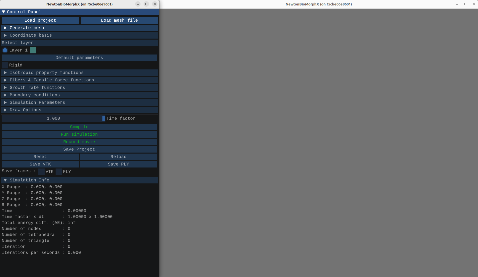
The graphical user interface with the control and rendering windows.
NewtonBioMorphX allows users to generate a new mesh directly within the GUI by selecting one of the six predefined primitive geometries:
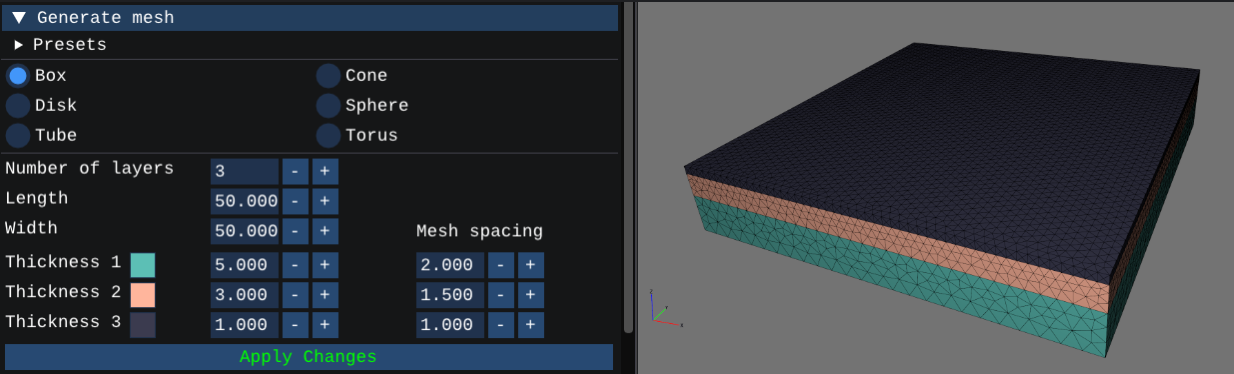
Generate mesh panel (left) and rendered result (right).
Smaller mesh spacing gives higher resolution but increases computation time. After entering the dimensions and the layer details, click Apply Changes to trigger the mesh generator. After a while, the result will appear in the rendering window.
NewtonBioMorphX includes twelve ready-to-run examples that illustrate the main mechanical processes available in this framework. These presets provide an excellent starting point for new users and illustrate how growth, elasticity, plasticity, fibre reinforcement, active contractility, multilayer interactions, and geometry collectively influence morphogenesis.
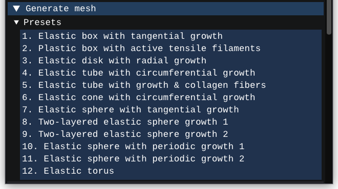
List of preset examples.
| Preset | Summary | Result |
|---|---|---|
| 1. Elastic Box with Tangential Growth | Demonstrates the emergence of self-organized surface folds and polygonal domains driven by isotropic tangential growth constrained by an underlying rigid substrate. | 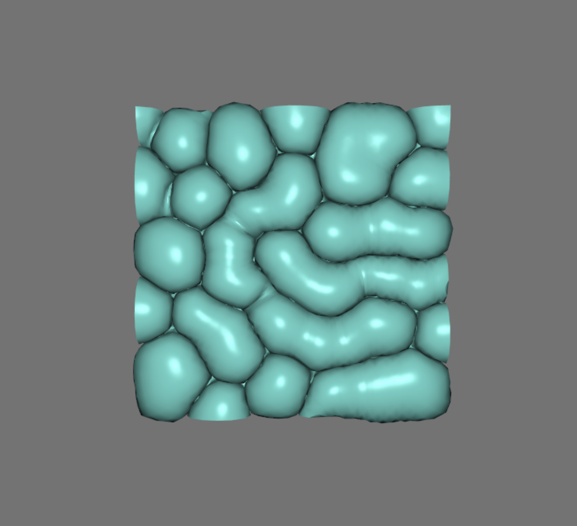 |
| 2. Plastic Box with Active Tensile Filaments | Shows how active contractile forces can reshape tissues in the absence of growth and generate large-scale deformations in a plastic material. | 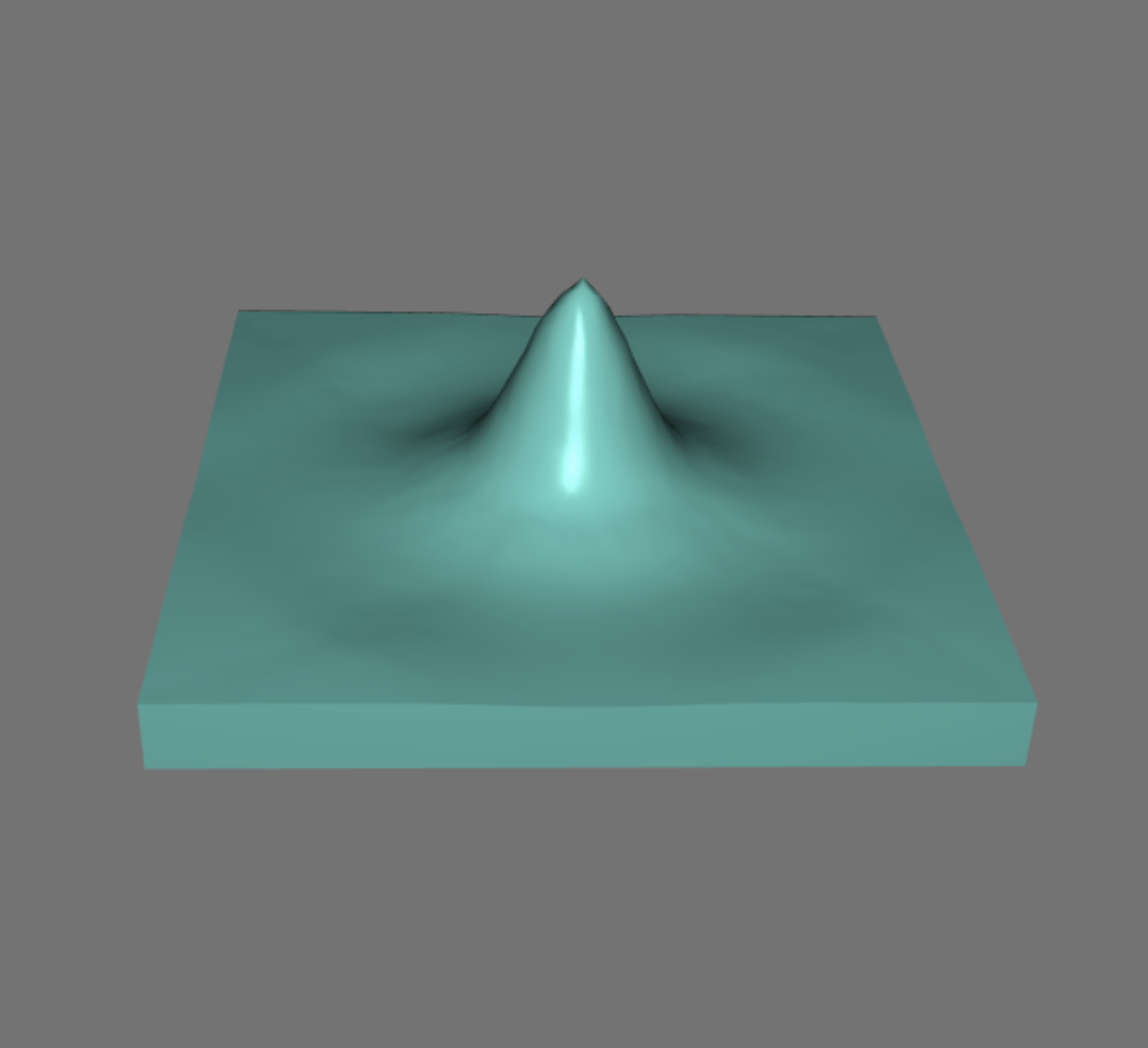 |
| 3. Elastic Disk with Radial Growth (Disk → Cone) | Illustrates the transformation of a flat disk into a conical geometry through differential radial growth. | 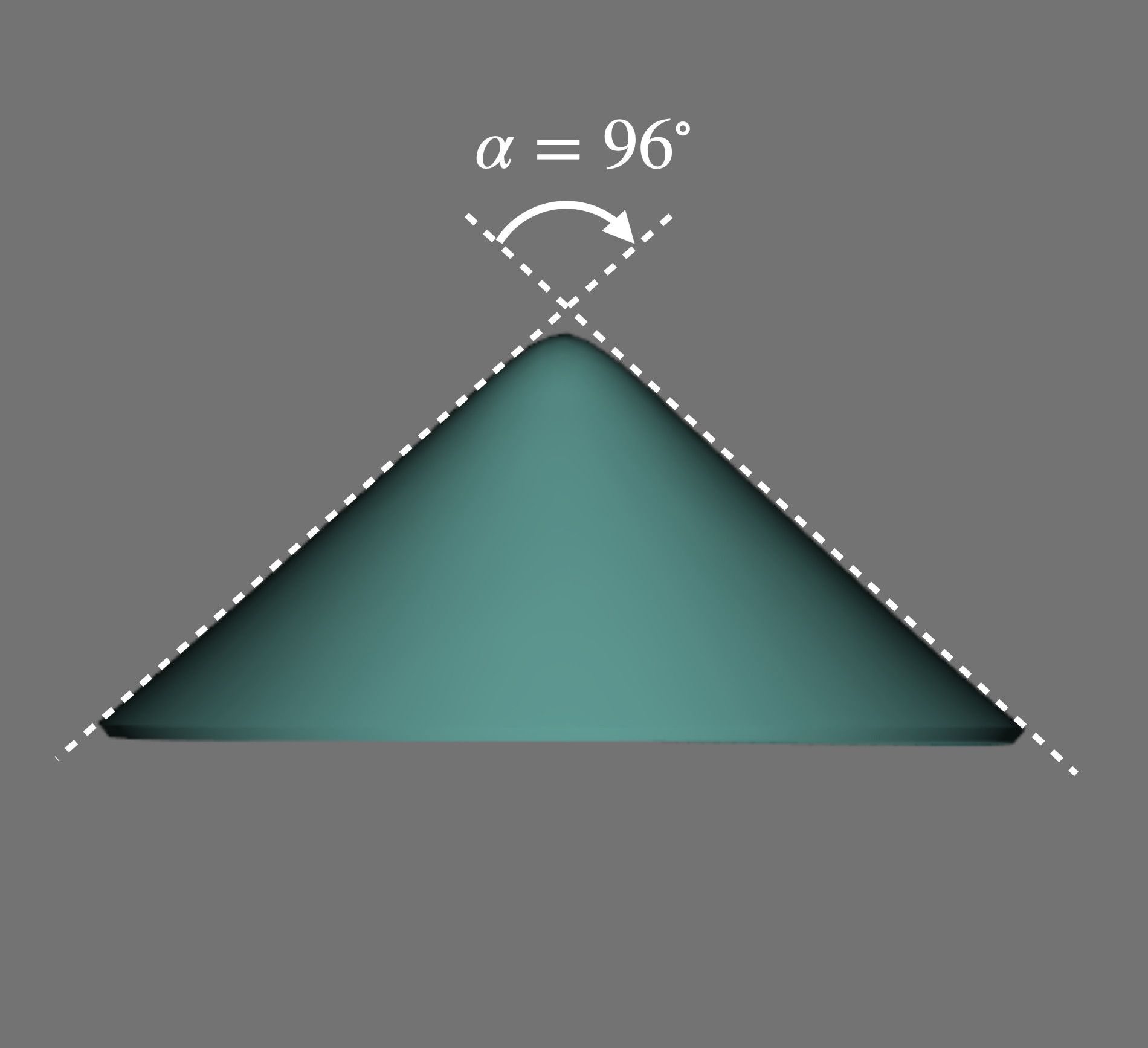 |
| 4. Elastic Tube with Circumferential Growth | Demonstrates longitudinal crease formation caused by circumferential growth in a cylindrical tissue. | 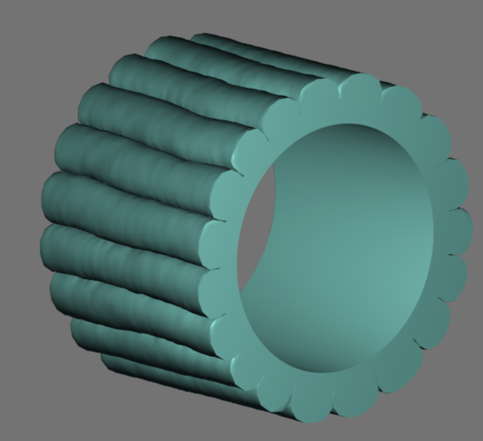 |
| 5. Elastic Tube with Growth and Collagen Fibres | Shows how anisotropic collagen-like fibres orient and guide surface folding, producing crocodile head-scale patterns. | 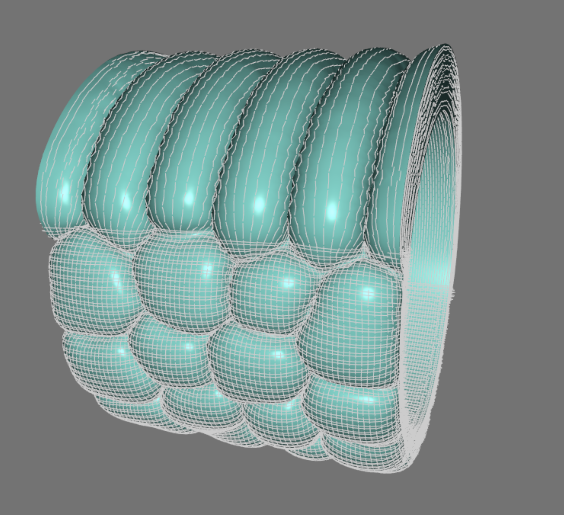 |
| 6. Elastic Cone with Circumferential Growth | Illustrates growth-induced folding on a conical surface and how fold number changes with local radius. | 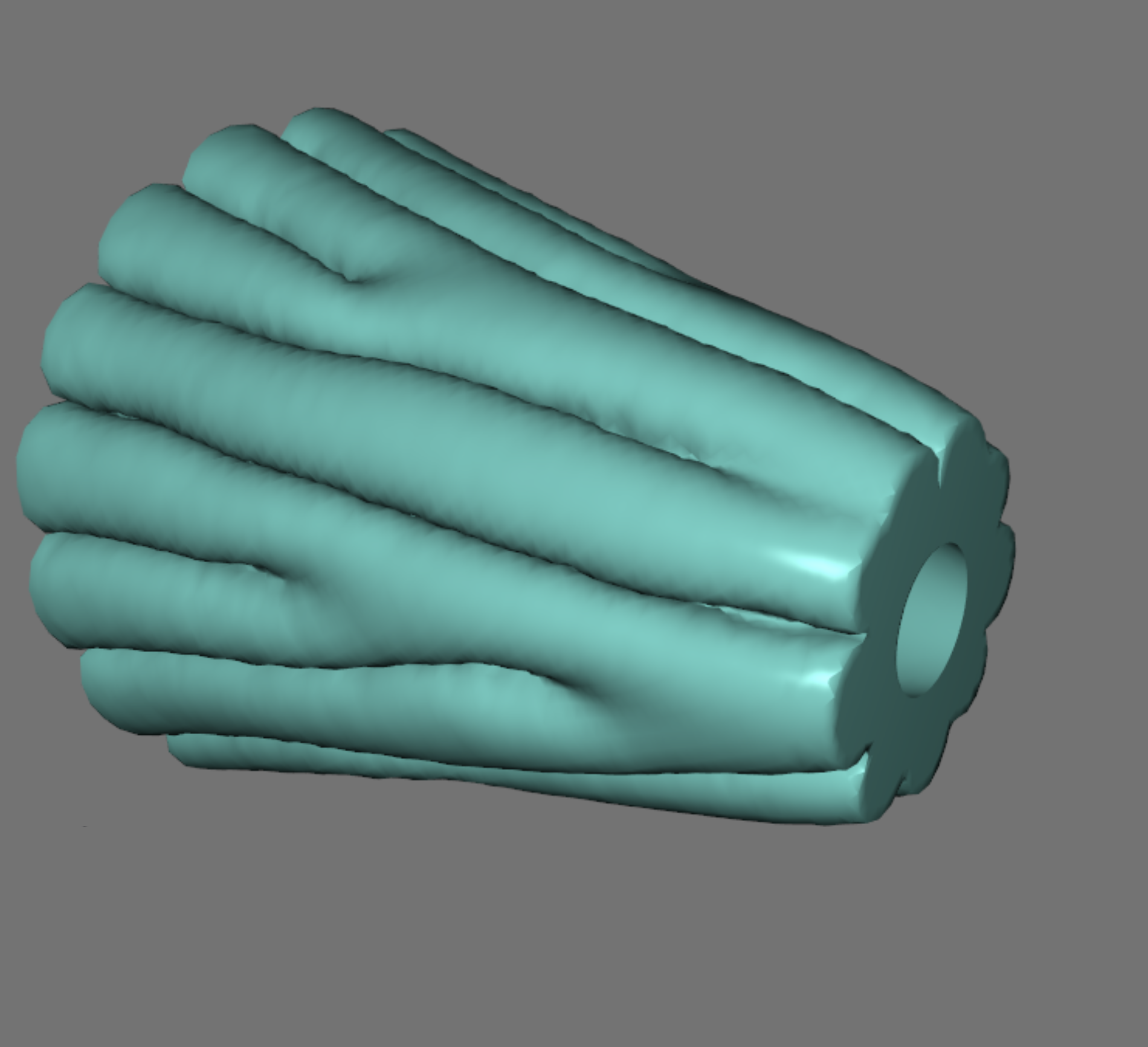 |
| 7. Three-Layer Sphere with Tangential Growth | Demonstrates multilayer mechanical interactions and the emergence of distinct folding length scales in different spherical layers. | 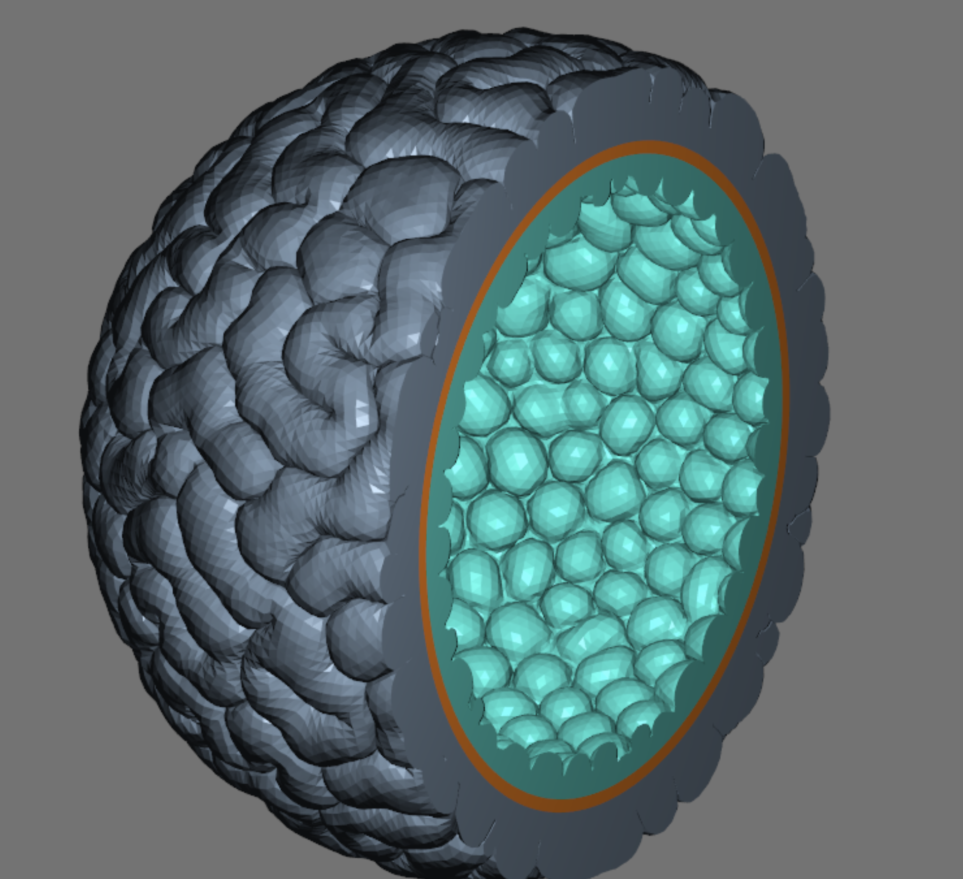 |
| 8. Two-Layer Sphere with Orthogonal Growth Directions | Shows symmetry breaking and the spontaneous formation of a pseudo-torus morphology resulting from competing orthogonal growth directions. | 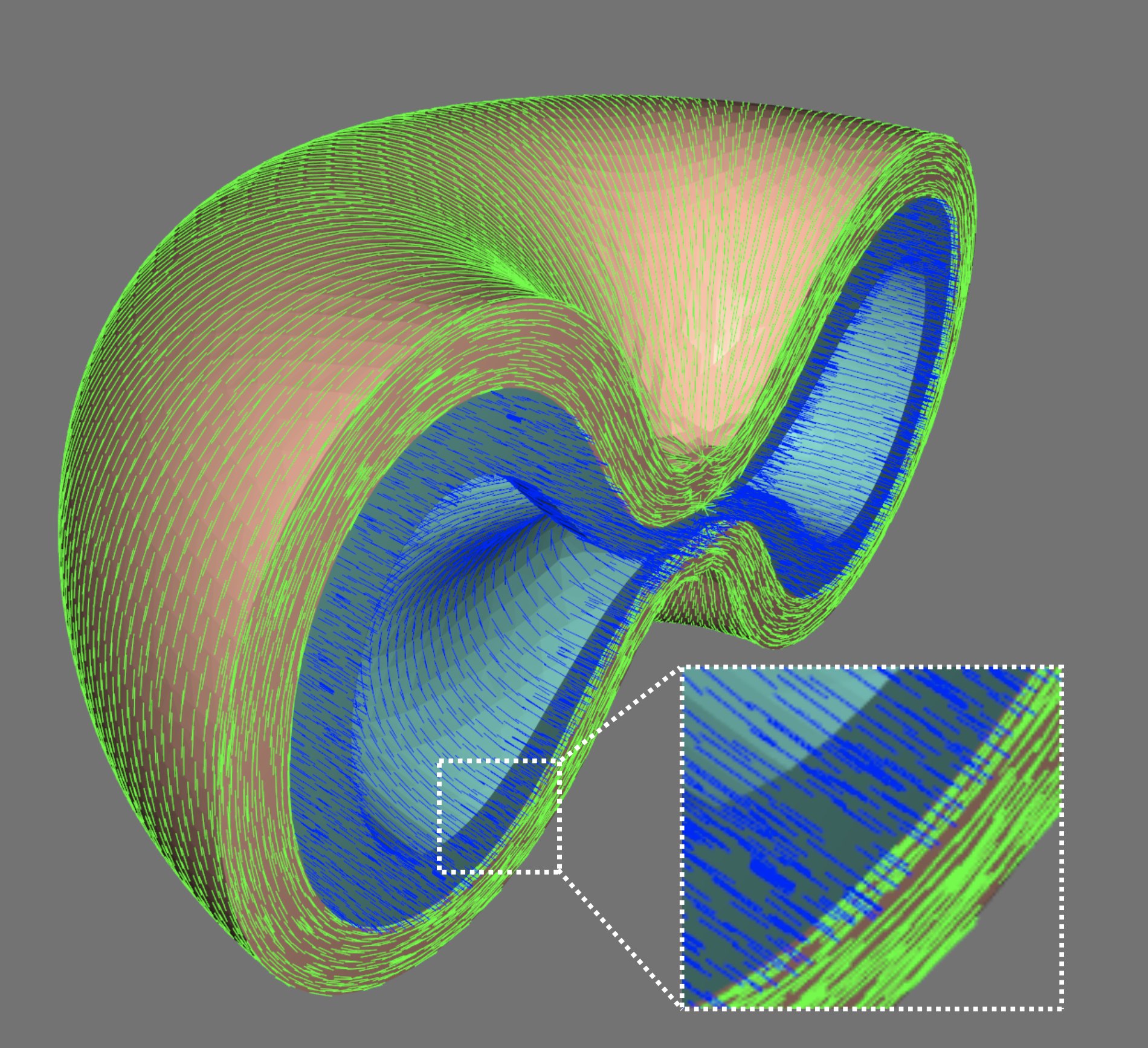 |
| 9. Two-Layer Sphere with Opposing Hemispheric Growth | Illustrates how spatially asymmetric growth can generate strongly polarized global deformations. | 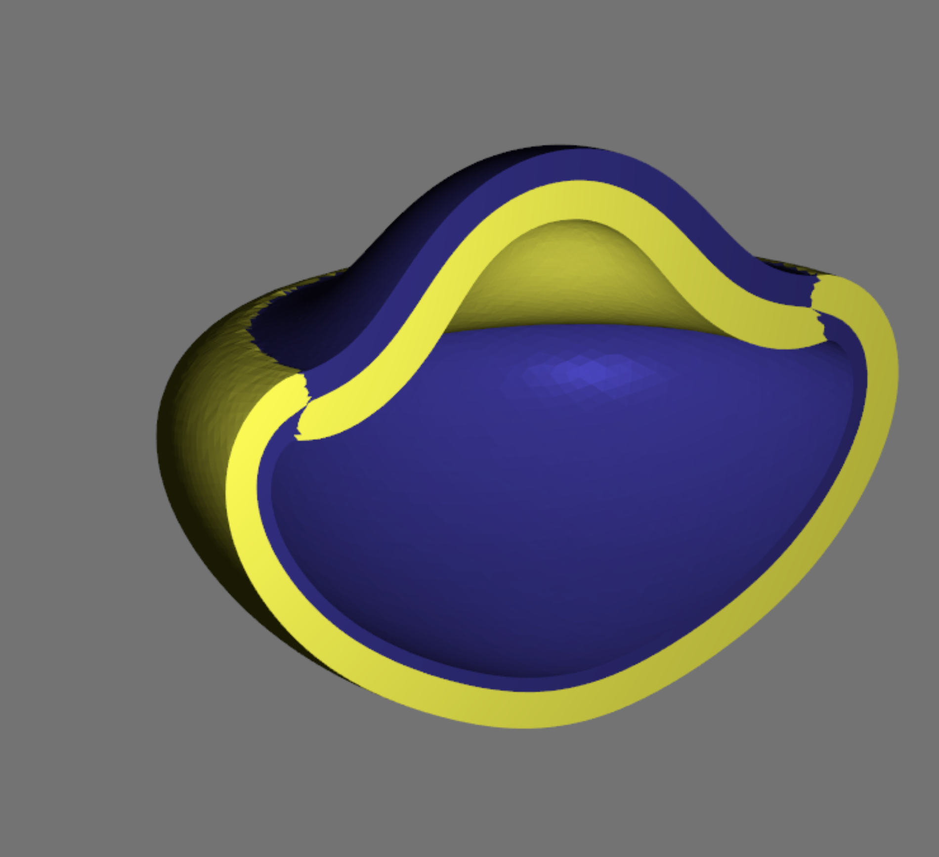 |
| 10. Sphere with Azimuthal Periodic Growth | Demonstrates the formation of regularly distributed surface domains driven by prescribed periodic growth patterns. | 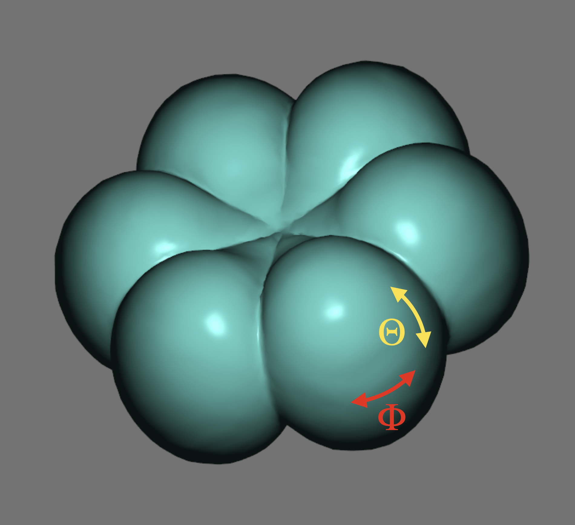 |
| 11. Sphere with Polar and Azimuthal Periodic Growth | Shows how combining multiple periodic growth fields produces highly patterned and anisotropic spherical morphologies. | 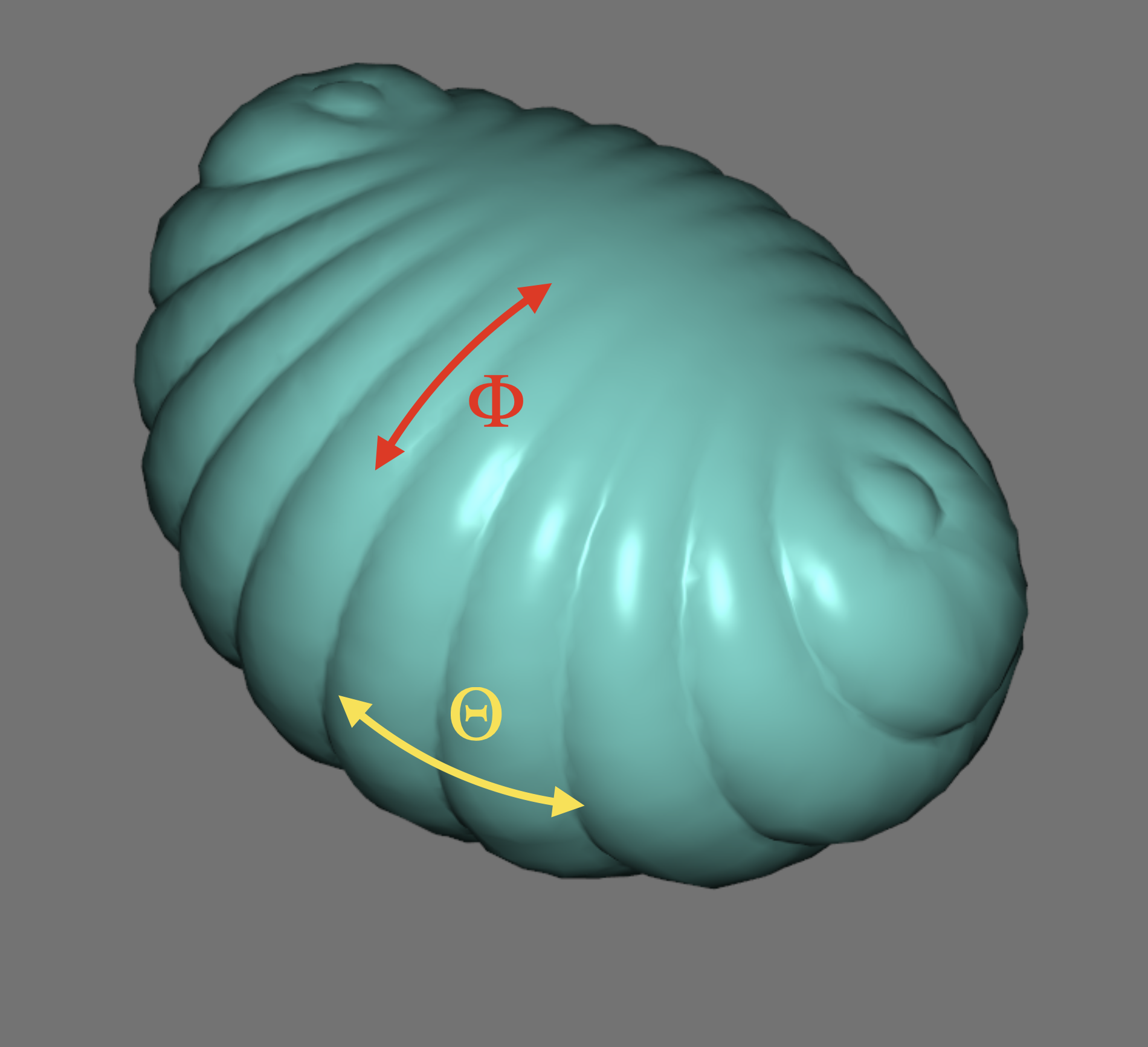 |
| 12. Elastic Torus with Fibres | Demonstrates self-organized polygonal folding on a toroidal geometry reinforced by orthogonal fibre families. | 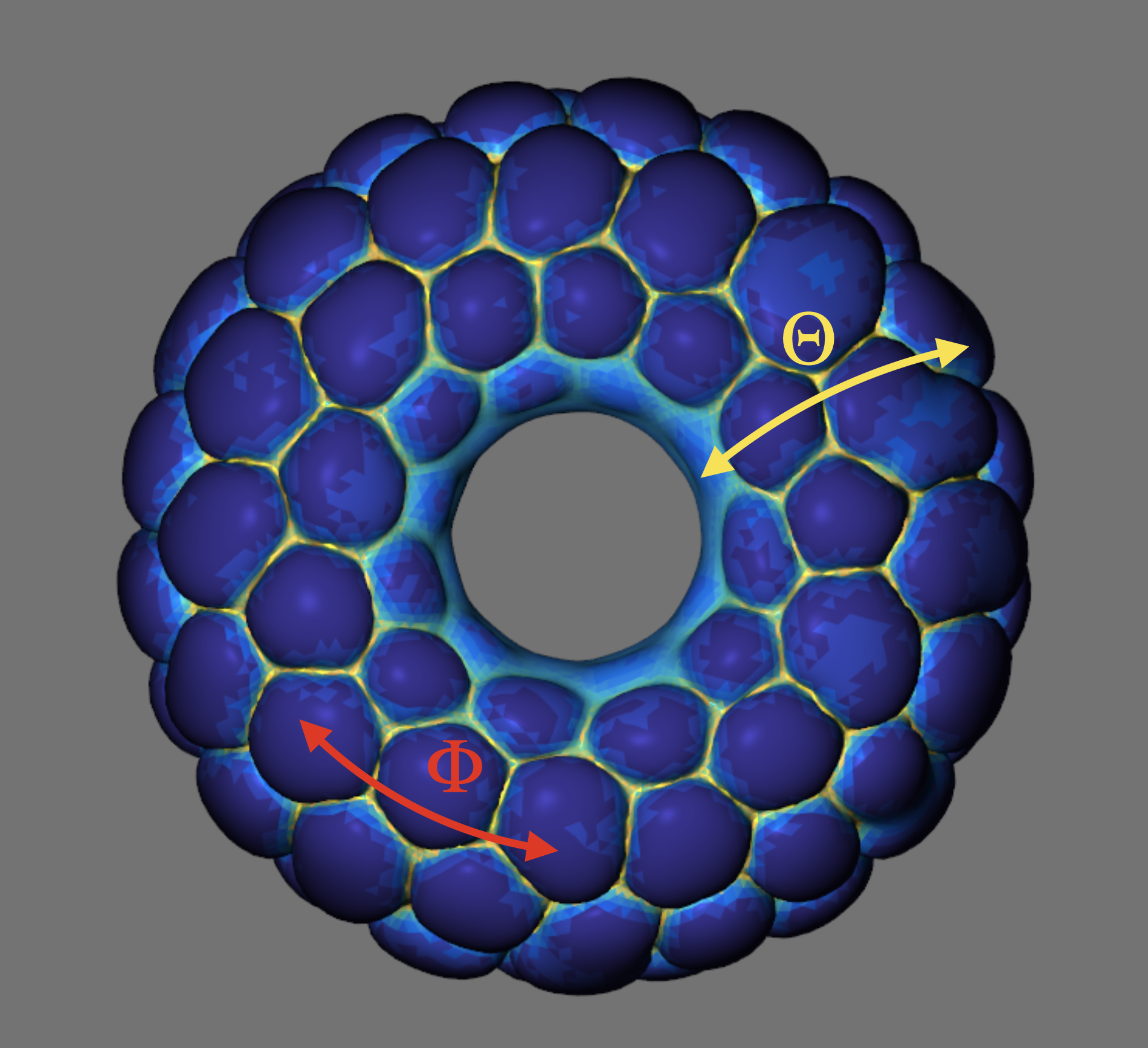 |
We encourage you to work through the twelve illustrative presets in order: together, they progressively introduce the major capabilities of NewtonBioMorphX.
The corresponding examples are described in detail in the original NewtonBioMorphX article (1). Users interested in reproducing the published examples exactly are encouraged to consult the original article together with the preset configuration files distributed with the software.
NewtonBioMorphX allows growth, fibres, active tensile forces, and boundary conditions to be defined in different coordinate systems. Choosing a coordinate system adapted to the geometry often simplifies model construction and makes biological interpretation more intuitive.
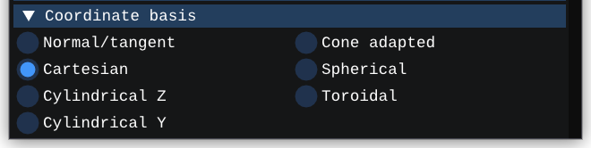
Coordinate Basis Panel.
The application allows for the use of the following coordinate systems:
Advanced reading: ‘Coordinate basis definitions’ in the appendix of our original NewtonBioMorphX article (1).
Many biological tissues consist of juxtaposed layers. NewtonBioMorphX allows the user to define different material properties — such as growth rates, stiffness, Poisson’s ratio, plasticity, and the distribution of fibres and active forces — for each layer.

Select Layer panel in which Layer 1 is marked as a rigid layer.
Note also that a layer can be marked as Rigid. In that case, the corresponding layer does not deform, does not grow, and ignores material-property definitions (hence, in that case, the corresponding panels are automatically disabled). Setting a layer as rigid is particularly useful for representing very hard tissues (such as bone) or artificial supporting substrates.
If a layer is not set as rigid, the panel below lets you define its isotropic material properties using mathematical expressions, with the syntax explained in Section 13. If the input mesh provides these properties as described in Section 23, you can instead read them from the mesh file by ticking the checkbox next to each corresponding property.
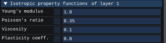
Isotropic material properties panel.
Advanced reading: ‘Material model and governing equations’ and ‘Plasticity’ sections in the original NewtonBioMorphX article (1).
Many biological tissues are mechanically anisotropic, meaning that they resist deformation differently depending on the direction. NewtonBioMorphX allows for the use of passive fibres and active tensile forces that endow some tissues with such anisotropies.
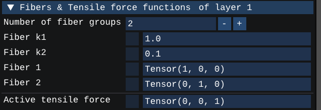
Fibers & active forces panel.
Passive fibres mimic collagen-like reinforcement. Up to four independent fibre families can be defined for each layer. The presence of fibres increases stiffness preferentially along their orientation and therefore influences the direction of tissue folding. The fibre parameters are:
Increasing either parameter strengthens the mechanical effect of fibres.
Fibre orientations and densities are specified by rank-one tensors. Tensor syntax allows defining any orientation. In the simplest cases, only one component of the tensor is non-zero. For example, Tensor(1,0,0) creates fibres aligned with the first direction of the coordinate basis (e.g., X in the Cartesian coordinates, or R in the spherical coordinates). Similarly, Tensor(0,0.5,0) creates fibres aligned with the second direction of the coordinate basis (e.g., Y in the Cartesian coordinates, or Θ in the spherical coordinates) and with one quarter (the square of 0.5) of the density in the first example.
More generally, Tensor(v1,v2,v3) represents a rank-one tensor defined by Vector(v1,v2,v3) times its transpose.
Active tensile forces mimic contractile biological structures such as actin filaments. Unlike passive fibres, active tensile filaments continuously generate stress within the tissue. In NewtonBioMorphX, these active forces can be set as:
Note that passive fibres and active contractile stresses can also be read from the input mesh (if they are provided as described in Section 23) by ticking the checkbox next to each corresponding property.
Advanced reading: ‘Material model and governing equations’ section in the original NewtonBioMorphX article (1).
Growth functions determine how the tissue expands. Growth are defined independently along each of the principal directions of the selected coordinate basis. Note that it could be argued that negative growth rates would correspond to tissues contracting over time through cell death; we, however, have never explored this possibility and advise using only positive growth rates.

Growth rates panel.
When the same growth rate is assigned to all directions, growth is isotropic. When different growth rates are assigned to different directions, growth is anisotropic. Here are some examples of values or functions that can be assigned to any of the coordinate components:
0.001: uniform and steady growth.
0.001*exp(-0.001*t): the initial growth rate of 0.001 decays exponentially with time. Note that the ratio between the initial growth rate (here, 0.001) and the decay rate (here, also 0.001) gives the amount of growth at steady state (here 100% because 0.001/0.001=1).
0.001*(1+X/50): the growth is varying in space, i.e., linearly with X. More specifically, if the domain is centered at zero and its size is 100, then the growth rate varies from 0 (at X=-50) to 0.002 (at X=50).
0.001*(X>0): if the domain is centered at zero, growth is restricted to half of the tissue.
Note that growth rates can also be read from the input mesh (if they are provided as described in Section 23) by ticking the checkbox next to each corresponding property.
Begin with small growth rates and progressively increase them, because too large a growth rate may generate deformations that are too rapid and cause numerical instabilities.
Advanced reading: ‘Growth, passive fibre, and active tensile filament dynamics’ section in the original article (1).
NewtonBioMorphX works in non-dimensional (simulation) units, with the mass density fixed at 1. To relate a simulation to a physical system, choose:
L, T and the material properties must be expressed in the same consistent unit system (e.g., the International System of Units —SI— in seconds, meters, kilograms). With ρ denoting the physical mass density, a simulation value is converted to physical units by multiplying it by the corresponding conversion factor in the table below. Conversely, to convert a physical value into a simulation value, divide by the same factor.
| Quantity | Conversion factor |
|---|---|
| Length | L |
| Time | T |
| Density | ρ |
| Young’s modulus, stress (including active stress), pressure, and k1 | ρ · L² / T² |
| Viscosity | ρ · L² / T |
| Rates (e.g. growth rate) | 1 / T |
For example, physical length = L × the number of length units indicated in the software. Conversely, the simulation Young’s modulus (E-sim) is equal to the corresponding physical value (E-phys) multiplied by T² / (ρ · L²). Note that the Poisson’s ratio (ν), the plasticity coefficient (χ), and strains are dimensionless quantities; their simulation and physical values are therefore identical.
For many soft tissues and hydrogels, ρ ≈ 1000 kg/m³, E-phys ≈ 1–100 kPa, and the viscosity η-phys ≈ 10–100 Pa·s (effective viscosity under slow deformation).
To simulate a material with ρ = 1000 kg/m³, E-phys = 100 kPa and η-phys = 50 Pa·s, any of the following choices can be used, where E-sim = E-phys · T² / (ρ · L²) and η-sim = η-phys · T / (ρ · L²):
| L | T | E-sim | η-sim |
|---|---|---|---|
| 0.1 m | 1 ms | 0.01 | 0.005 |
| 1 cm | 1 ms | 1 | 0.5 |
| 1 mm | 1 ms | 100 | 50 |
In other words, the second line corresponds to a choice of centimetres and milliseconds as the simulation length and time units; one simulation unit of Young’s modulus then corresponds to 100 kPa, and 0.5 units of the viscosity coefficient correspond to 50 Pa·s.
Biological growth is typically much slower than the mechanical response of the material. With the units above, the mechanical timescales are milliseconds, whereas growth takes minutes to days. However, simulating growth at those true physical rates is unnecessary and computationally too expensive. All we need to ensure is that the material is in mechanical equilibrium at every stage of growth (i.e., a quasi-static regime). In particular, if you are interested in recapitulating the dynamics of the system (i.e., its valid intermediate states), you should choose a growth rate small enough that the characteristic growth time (≈ 1 / growth rate, i.e., the simulation time over which the material grows by about 100%) is 10–100 times longer than the slowest mechanical timescale. The slowest mechanical timescale is the larger of the inertial time (≈ specimen size / √E-sim, in simulation units) and the viscous time (≈ η-sim / E-sim).
Note that you can check for convergence by halving the growth rate and confirming that the resulting pattern does not change (this is especially important if the material undergoes plastic deformation).
Boundary conditions determine how tissue surfaces move and how external forces act on them. NewtonBioMorphX supports four types of boundary conditions described below.
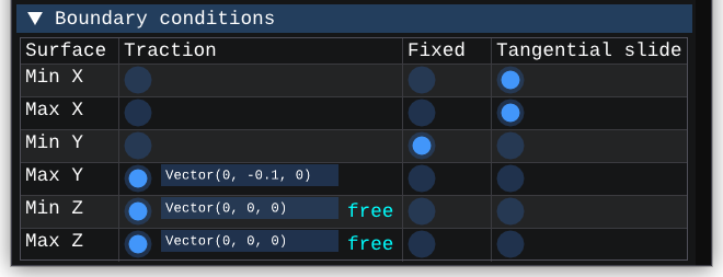
Boundary conditions panel.
A traction boundary condition applies an external force per unit area to a surface. Users may specify the traction analytically, as in the following examples:
Vector(0,0,1)Vector(0,10*sin(t/100),0)Vector(0,R,0)Traction boundary conditions are useful for externally loaded tissues and classical solid-mechanics benchmarks such as Cook’s membrane.
A free boundary is a special case of traction where the applied force is zero everywhere (Vector(0,0,0)). The surface can therefore move freely under the action of internal forces. This is typically the condition assigned to folding tissue surfaces.
Displacement is completely prevented. This condition is especially useful for modeling tissues anchored to rigid tissues (such as bone) or artificial rigid substrates. Note that it is therefore a convenient (and more efficient) alternative to the assignment of an underlying rigid layer (see Section 7).
Motion parallel to the surface is allowed while motion normal to the surface is prevented. This condition is particularly useful for modeling sliding interfaces even if the corresponding boundary is curved (such as the internal boundary of a cylinder or a sphere).
Advanced reading: ‘Time integration and boundary conditions’ and ‘Boundary forces’ sections the original NewtonBioMorphX article (1).
All the parameters used to define material properties, fibres, active forces, growth rates, and traction boundary conditions (Sections 8,9,10 and 12) can be entered as analytical expressions using the following available variables:
X, Y, Z : reference coordinate components used in the Cartesian and tangential-normal bases;R : reference radial component used in spherical, cylindrical, or toroidal bases;Theta (Θ): reference angular, polar, or poloidal component used in cylindrical, spherical, or toroidal bases;Phi (Φ): reference azimuthal or toroidal component used in spherical or toroidal bases;t : time.Note that all these coordinates correspond to the reference configuration (i.e., at t=0). In other words, these are co-deforming coordinates.
The available operators are: +, -, *, /, < , >, == (equal), and != (not equal).
The available functions are: sin(), asin(), sinh(), cos(), acos(), cosh(), tan(), atan(), atan2(), tanh(), exp(), log(), sqrt(), pow(), and abs().
Vector expressions, such as Vector(1,0,0), are useful for defining traction boundary forces as discussed above in Section 12.
Rank-one tensor expressions, such as Tensor(1,0,0), are useful for assigning fibre orientations and active forces, as discussed in Section 9.
The Simulation Parameters panel controls how the numerical solver behaves during the simulation. These settings do not define the biological model itself but rather determine how the software computes and stabilizes the solution.
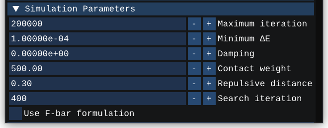
Simulation parameters panel.
For most users, the default values provide a good starting point. However, understanding these parameters can greatly improve simulation robustness and performance.
This parameter specifies the maximum number of solver iterations that can be executed before the simulation automatically stops.
Use a larger value when growth is slow, when large deformations are expected, or when the simulation has not yet reached a stable state.
Use a smaller value when testing a new model or quickly exploring the effects of changing parameter values.
This parameter controls the automatic stopping criterion. NewtonBioMorphX continuously monitors how much the mechanical state changes over time. Once those changes become sufficiently small, one can consider that the simulation has converged.
Use larger values for faster simulations and earlier termination, with the risk of not reaching the steady state. Use smaller values for more accurate steady states (at the cost of longer computation time). We recommend using the default value for routine simulations and decreasing it when publication-quality results are required.
Damping removes mechanical motion and accelerates convergence toward equilibrium. Without damping, some models can oscillate for a long time before reaching a stable configuration.
Use higher damping for smoother evolution and to avoid oscillations. Use lower damping for more realistic transient dynamics, at the cost of longer running time. Importantly, while it can be very useful for purely elastic problems (because the same steady state will, in principle, be reached whatever the damping value), damping is likely to alter the final solution when tissues are undergoing plastic deformations. Note that viscosity also dampens the simulation (by mitigating short wavelength oscillations) and will also affect the final results when tissues undergo plasticity. However, viscosity is an actual property of materials, whereas the damping parameter discussed here is a numerical trick that should be used with caution.
The contact weight controls the strength of collision forces used to prevent different parts of the tissue from penetrating each other.
Use higher values for a stronger response to collisions (to the potential cost of smaller stable time steps). Use lower values for a softer response to collisions (and potentially larger stable time steps) but the risk of observing non-physical interpenetrations.
This parameter determines how close two surfaces must be before contact forces become active. It may be viewed as an interaction thickness around the tissue.
Use larger values for earlier contact detection and stronger prevention of self-intersections (at the cost of potentially more contact events). Use smaller values for later contact detection with the risk of observing non-physical interpenetrations. We recommend using the default value unless contact artefacts become visible.
NewtonBioMorphX periodically searches for nearby surfaces that may come into contact. This parameter controls the amount of computational effort devoted to collision detection.
Use larger values for a more exhaustive contact search and better handling of complex folding. Use smaller values for faster simulations with the risk of missing contacts. We recommend increasing the search-iteration value only for highly folded tissues or geometries with extensive self-contact.
The F-bar formulation is a specialized numerical technique that greatly reduces the risk of the so-called ‘volumetric locking’ artefact that affects the accuracy of simulations when nearly incompressible materials are involved. It is therefore advised to select the ‘F-bar formulation’ checkbox for Poisson’s ratios higher than 0.45.
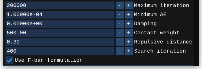
F-bar checkbox.
The Cook’s membrane benchmark included in the original NewtonBioMorphX article (1) demonstrates the advantages of the F-bar formulation for nearly incompressible materials.
For growth-driven morphogenesis, use:
For strongly folded tissues:
For nearly incompressible materials, use F-bar formulation.
Advanced reading: Users interested in better understanding the effects of varying simulation parameters are encouraged to consult the following sections in the original NewtonBioMorphX article (1):
The Draw Options panel controls how simulation results are displayed. It allows users to inspect the external and internal geometries, as well as the mechanical state and properties of the tissues.
More specifically, the visualization system is designed to help users understand how the tissue deforms, how growth is distributed, where stresses accumulate, how fibres deform, how active contractile filaments are oriented, how tetrahedra are distributed, and whether the numerical mesh remains of good quality.
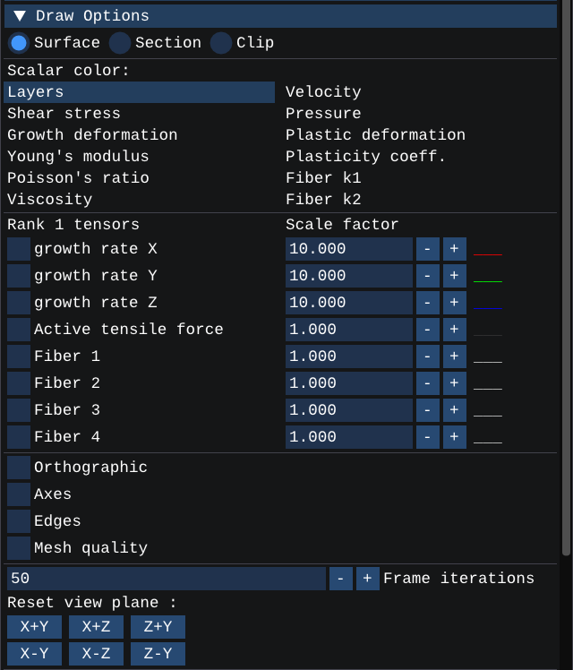
Draw Options panel.
The three visualization modes determine which portion of the geometry is displayed.
The Surface mode displays the external boundary of the tissue. This is the most commonly used visualization mode and is ideal for observing global shape changes, studying wrinkles and folds, producing images and movies, and analyzing final morphologies.
The Section mode displays a cross-section of the volume. Available section directions are X, Y, and Z planes. The plane position can be adjusted continuously using the corresponding sliders. Typical applications are:
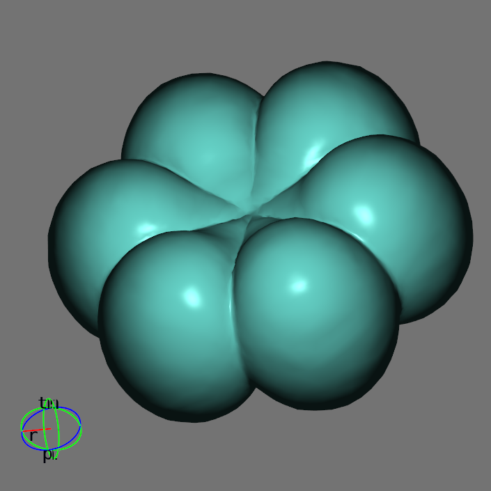
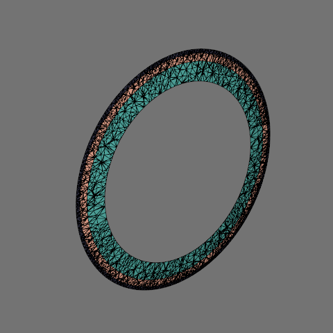
The rendered model in Surface mode (left) and Section mode with mesh edges (right) is displayed.
The clipping direction can be inverted by selecting the Invert checkbox to compare opposite sides of a model. This allows users to inspect either side of the clipping plane. If the Crinkle Clip checkbox is selected, crinkle clipping preserves the original surface elements intersected by the clipping plane. One typical application of the crinkle clipping mode is to inspect the mesh structure for identifying highly distorted tetrahedra.
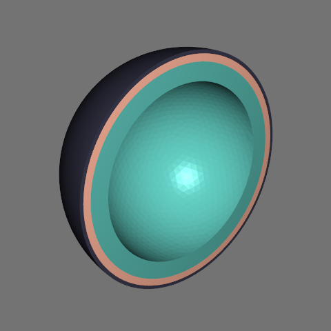
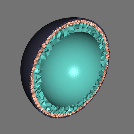
The rendered model in Clip mode (left) and Crinkle Clip mode (right).
A scalar field assigns one numerical value to each region of the tissue. NewtonBioMorphX displays scalar fields using color maps. By default, low and high values appear in dark and bright colors, respectively. All of the quantities listed below are useful to monitor during the simulation. The current range of values is dynamically updated in the color bar displayed next to the model. The following scalar fields can be displayed:
Layer: Displays the layer identity to observe multilayer geometries and identify tissue boundaries.
Shear Stress: Displays the von Mises stress, which measures mechanical shear loading independent of direction.
Plastic Deformation: Displays the accumulated permanent deformation to identify yielding zones.
Growth Deformation: Displays the local amount of accumulated growth.
Young’s Modulus: Displays the distribution of stiffness (Young’s modulus).
Poisson’s Ratio: Displays the distribution of Poisson’s ratio, i.e., of the degree of incompressibility.
Viscosity: Displays the distribution of the viscosity coefficient.
Velocity: Displays the magnitude of node velocities; useful for identifying deforming zones and monitoring convergence.
Pressure: Displays volumetric stress within the domain. Positive/negative values indicate regions under compression/tension. Pressure visualization is particularly useful when testing the F-bar formulation.
Plasticity: Displays the distribution of the plasticity coefficient.
k1 and k2: Displays the distribution of fibre stiffness parameters k1 and k2.
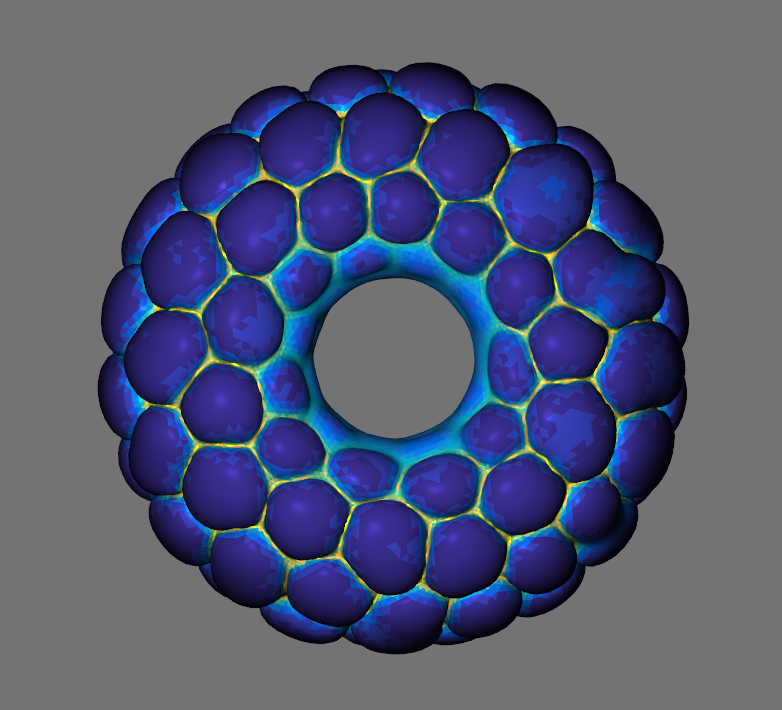
The rendered model with the pressure Scalar Field displayed in surface mode.
Users can visualize the following rank-one tensor fields as line elements:
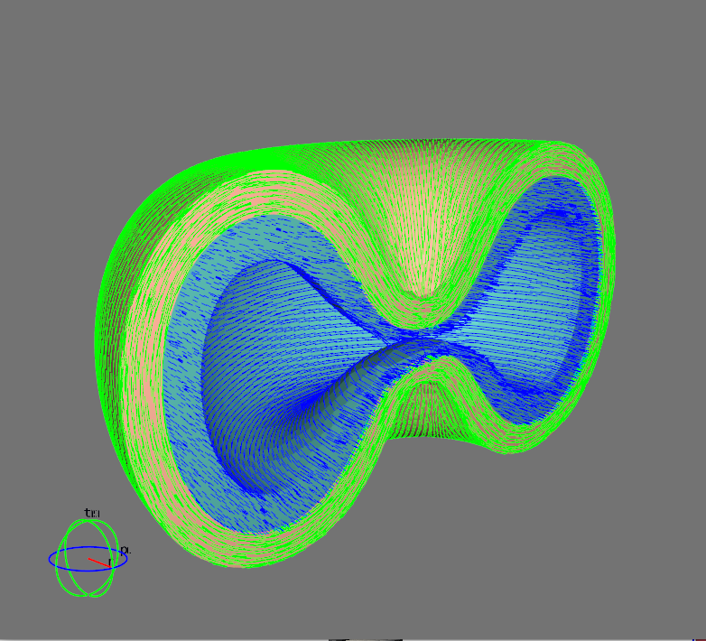
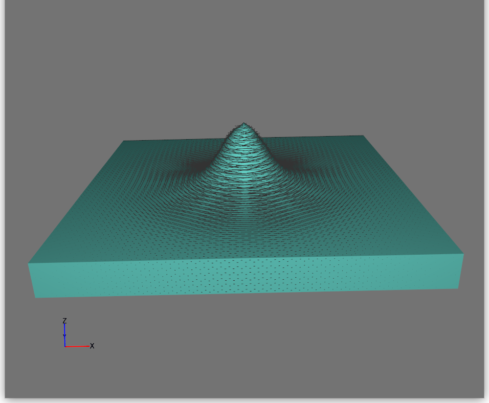
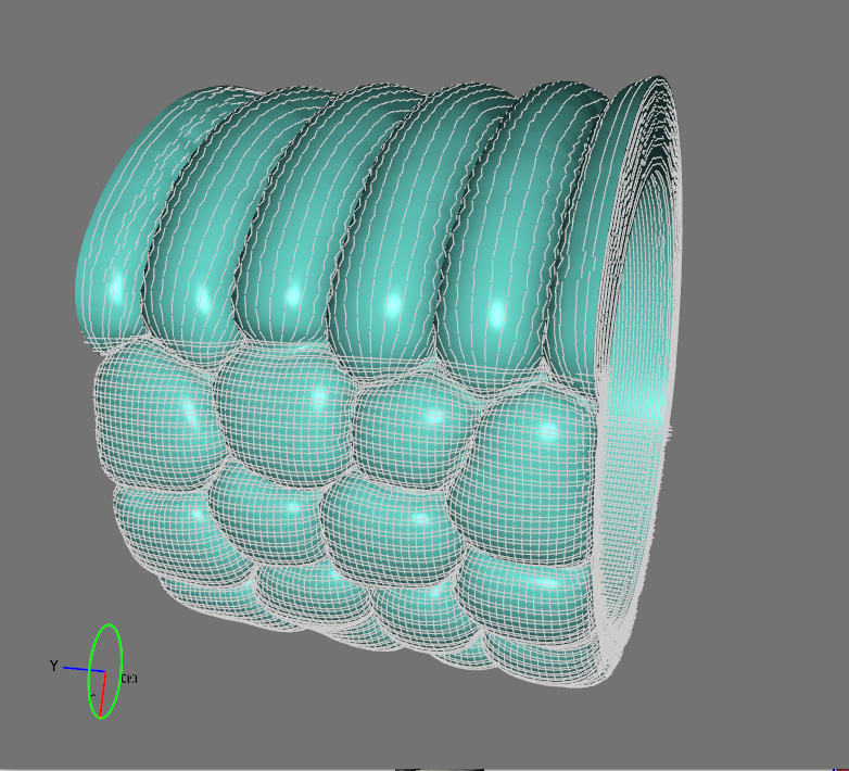
Note that the user can also choose to display the model in ‘Perspective’ or ‘Orthographic’ projection. Other options available are to show or hide mesh edges and the axes of the selected coordinate basis. Finally, a normalized histogram (with adjustable bins) can be displayed for monitoring mesh quality; it ranges from 0 (corresponding to ill-posed zero-volume tetrahedra) to 1 (perfectly regular tetrahedra). Values below 0.2 and 0.05 are shown in yellow and red, respectively. When a large proportion of tetrahedra exhibit values below 0.05, distortions are too large for trusting the numerical result.
Frame iterations defines the frequency at which the current simulation state is shown in the rendering window, while the Reset view plane buttons allow orienting the geometry along any of the six Cartesian viewing directions; this functionality is particularly useful to ensure comparable orientations of different simulation results.
NewtonBioMorphX continuously monitors numerical stability during execution. If instability is detected, the simulation automatically returns to the last stable state and the time step is reduced. This ensures that the simulation is performed with stable time steps. This functionality greatly improves robustness when exploring new parameter combinations.

Time Factor panel.
Note that the user can manually tune the Time Factor parameter to exert direct control over simulation speed and numerical stability. Higher values allow for faster progression through simulated time but increase the risk of numerical instability. Lower values improve numerical stability at the cost of a slower simulation.
We recommend keeping the value at 1.0 unless NewtonBioMorphX updates it automatically.
Once the geometry, material properties, growth laws, fibre architectures, and boundary conditions have been configured, the simulation can be launched.

Compile and Run Simulation buttons.
Press Compile to generate the CUDA runtime kernels corresponding to the current model configuration. Compilation is required whenever parameters affecting the mechanical model have been modified, including:
Note that the Run simulation button becomes accessible only if compilation is successful. An unsuccessful compilation is most often due to errors in parameter functions introduced by the user.
Press the Run Simulation button to start the numerical computation. During execution, the geometry and all associated fields are updated in real time in the rendering window. While the simulation is running, users may:
Once the simulation starts, the Run Simulation button automatically changes to Pause Simulation. Press that button at any time to temporarily stop the computation.
The simulation stops automatically when the Energy Difference Tolerance (Minimum ΔE) criterion is reached (see Section 14) or when the maximum number of iterations has been exceeded.
NewtonBioMorphX provides several tools for saving the simulation project, exporting results, recording movies of the simulation dynamics, and restoring the initial state of a model.
Saving results, exporting data, and resetting simulation options.
This functionality makes it possible to produce an MP4 movie directly from the rendering window. Press Record Movie to begin recording.
While recording is active:
Generated video files are automatically saved in the application root directory using the following file names: output_0.mp4, output_1.mp4, output_2.mp4, …
Clicking on this button opens a file-selection dialog for storing the complete simulation setup in a project file. The saved project includes:
Project files are stored in plain-text (.txt) format and can later be reloaded using the Load Project button (see Section 3).
The Reset button restores all simulation variables to their initial state defined in the project file. The Reload button is useful if the user wants to reload a new geometry (from a mesh file with the same file name as the one previously loaded) while keeping all current simulation variables unchanged.
This button allows exporting the current mesh, for example, for visualization in other software (such as ParaView, VisIt, or Python post-processing workflows). Note that the exported VTK file includes the current mechanical state as well as the current simulation variables:
This is useful if the user wants to visualize in other applications not only the mesh but also some of these attributes.
This button allows exporting the current surface mesh in PLY format. PLY files primarily contain geometric information and are intended for surface visualization and rendering software such as Blender and MeshLab.
Frame export automatically saves simulation snapshots during execution. The supported formats are VTK and PLY. Saved files are written automatically to the application root directory using the following file names:
output_0.vtk, output_1.vtk, output_2.vtk, …output_0.ply, output_1.ply, output_2.ply, …The Simulation Information panel provides real-time feedback about the current state of the simulation. It is a monitoring and diagnostic tool that helps users evaluate convergence, detect numerical issues, and understand the progression of the simulation.
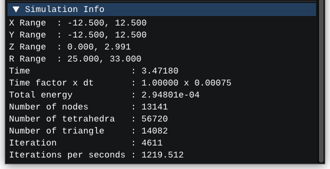
Simulation information panel.
Time displays the current simulation time, while Time factor x dt displays the effective time step. Note that it is the product of the Time Factor and the inherent time step dt.
dt is the time step estimated by NewtonBioMorphX on the basis of material parameters (such as Young’s modulus) and mesh resolution before the simulation is launched. The objective is to prevent numerical instabilities from occurring. Because the mesh can deform and material parameters can change over time (if time functions have been defined by the user), dt is dynamically re-evaluated at each time step.
Although dt is estimated such that numerical instabilities are unlikely, they can nevertheless occur in some situations (especially because of contacts during folding). This is when the Time factor becomes useful. Indeed, as indicated in Section 16, this scaling factor is updated by the software (or manually controlled by the user) when numerical instability is detected.
Together, Time factor and dt ensure stable effective simulation time increments.
Note that a rapidly decreasing time step can indicate that the model is approaching a numerically challenging configuration. An extreme example would be the deformation of a highly plastic material, thereby generating ill-posed tetrahedra.
This quantity displays the total Energy Difference (ΔE) metric used by NewtonBioMorphX as an indication of simulation convergence (see Section 14). Indeed, as a simulation approaches equilibrium, this quantity should decrease toward zero.
These quantities are constant during a simulation.
These two quantities display the number of solver iterations already performed and the current computational performance of the FEM solver, respectively.
In most cases, this occurs because the model has not been compiled. Press Compile and wait until the compilation completes successfully.
The convergence criterion may already be satisfied. In that case, try increasing the maximum number of iterations or decreasing the energy tolerance.
This might occur because:
Possible causes:
Try increasing Mesh spacing (see Section 4) or reducing Frame iterations (see Section 15).
If numerical instabilities persist, try to:
This artefact (volumetric-locking, see F-bar formulation) is likely to occur when using nearly incompressible materials. To avoid this artefact, try one of the following:
We encourage users to work through the twelve illustrative presets in order: together, they progressively introduce the major capabilities of NewtonBioMorphX.
If you prefer to compile NewtonBioMorphX yourself (for example, to target a specific GPU architecture or to modify the code), follow the instructions below for the Linux or Windows operating system. In both cases, the build is configured with CMake (version 3.21 or newer), and cmake --install produces a ready-to-use package. An internet connection is needed during the first configuration, as some dependencies (e.g., libigl) are downloaded automatically.
The Linux version is built inside a Docker container, defined by the Dockerfile in the repository. It provides the CUDA Toolkit and all required libraries, so the only prerequisite is the Docker engine.
From the project root, build the image and start the container:
docker build -t newtonbiomorphx .
docker run --rm -it -v "$PWD:/workspace" -w /workspace newtonbiomorphx
Then, inside the container, configure, build and package the application:
cmake -S . -B build -DCMAKE_BUILD_TYPE=RelWithDebInfo
cmake --build build -j
cmake --install build
The result is written to the install/ folder of the project:
install/AppDir/usr/: the application with its bundled libraries;install/NewtonBioMorphX-<version>-x86_64.AppImage: the single-file package (see Section 2).The following tools are required:
vcpkg install ffmpeg sdl2 vtk eigen3 gmp mpfr pkgconf --triplet x64-windows
From the project root, in a ‘Developer PowerShell for VS 2022’, type:
cmake -S . -B build -DCMAKE_TOOLCHAIN_FILE=<vcpkg>/scripts/buildsystems/vcpkg.cmake -DGMSH_ROOT=<path to gmsh SDK>
cmake --build build --config RelWithDebInfo
cmake --install build --config RelWithDebInfo
The application, with all required DLLs, is written to install/, and the packages to install/packages/: a portable .zip and, if NSIS is installed, an .exe installer.
By default, the code is compiled for the GPU architecture set in CMakeLists.txt. To target other GPUs, pass the corresponding compute capabilities when configuring, for example:
cmake -S . -B build -DCMAKE_CUDA_ARCHITECTURES="75-real;86-real;89-real;90-real;90-virtual"
Common values are 75 (Turing), 80/86 (Ampere), 89 (Ada Lovelace) and 90 (Hopper). The 90-virtual entry embeds portable code that newer GPUs compile at first launch. After changing the architecture, rebuild from a clean build directory.
NewtonBioMorphX can be run from the command line without launching the graphical user interface. This is particularly useful for running batches of simulations. To run a simulation, call the NewtonBioMorphX executable followed by the path of a project file:
NewtonBioMorphX path/to/project_file
The project file can either be generated from the graphical user interface, as explained in Section 18, or written by hand. It is a plain-text file that must contain:
saveTime parameter, which sets the time interval at which results are saved (used only in command-line mode);It may also contain:
The file must follow these rules:
Layer n, that is, all keys after that line, up to the next Layer line, apply to layer n.// on a line is treated as a comment and is ignored.\.For example, the following project file reproduces the gradient plot of tangential growth vs. passive fibres’ relative angle described in the original NewtonBioMorphX article (1):
inputGeom Arbitrary    // accepted values: Arbitrary, Box, Disk, Tube, Cone, Sphere, Torus
coordSystem Cartesian
inputMeshFileName input_mesh  // mesh of a 100 × 100 × 1 box
nLayers 1
nFibers 2
outputFileName output  // base name used for all output files

savePLY 1
saveTime 50

Layer 1
    isRigid 0

    // isotropic property functions
    nu 0.3333333
    E  1.0
    visc 0.01
    plasticity 0.0

    // growth rate functions
    grRate1_Ref 0.005 * exp(-t*0.005) * (0.75 + (Y+50.0)/100.0)
    grRate2_Ref 0.005 * exp(-t*0.005) * (0.75 + (Y+50.0)/100.0)
    grRate3_Ref 0.0

    // passive fiber stiffness and directions
    k1 0.1
    k2 0.0
    fiber1_Ref Tensor(1, 0, 0)
    fiber2_Ref Tensor((50.0-X) / sqrt((50.0-X)*(50.0-X) + (X+50.0)*(X+50.0)), \
                      (X+50.0) / sqrt((50.0-X)*(50.0-X) + (X+50.0)*(X+50.0)), 0)

    // active contractile force
    actin_Ref Tensor(0, 0, 0)
Project files reproducing other preset examples (Section 5) are provided in the examples folder.
NewtonBioMorphX can read tetrahedral meshes in VTK format (binary or ASCII). If the user wishes to provide more than the geometry, the file can also carry any of the following cell-data arrays:
CellEntityIds or layer: integers, one per tetrahedron, specifying the tissue layer to which it belongs.E: scalars, one per tetrahedron, giving its Young’s modulus.nu: scalars, one per tetrahedron, giving its Poisson’s ratio.viscosity: scalars, one per tetrahedron, giving its viscosity coefficient.plasticity: scalars, one per tetrahedron, giving its plasticity coefficient.grRate1, grRate2, grRate3: scalars, one per tetrahedron, giving its growth rate along each of the three coordinate basis directions.fiber1Tetra, fiber2Tetra, fiber3Tetra, fiber4Tetra: tensors (nine components: xx, xy, xz, yx, yy, yz, zx, zy, zz), one per tetrahedron, specifying the orientation of each of the four passive fibre families in the reference configuration.k1, k2: scalars, one per tetrahedron, giving its passive fibre stiffness parameters.actinTetra: tensors (nine components: xx, xy, xz, yx, yy, yz, zx, zy, zz), one per tetrahedron, specifying the contractile active stress in the reference configuration.If any of these properties is absent from the file, the user can still define in the user interface, using the corresponding expression field (with syntax defined in Section 13).